Fully Connected Network in PyTorch

Implementing a fully connected neural network in PyTorch

This page contains my notes on how to implement a fully-connected neural network (FCN) in PyTorch. It’s meant to be a bare-bones, basic implementation of an FCN.

What is an FCN?

A fully connected network (FCN) is an architecture with a bunch of densely-connected layers stacked on top of one another. In this architecture, each node in layer i is connected to each node of layer i+1, etc, with the output of each layer being passed through an activation function before being sent to the next layer. Here’s what this looks like:

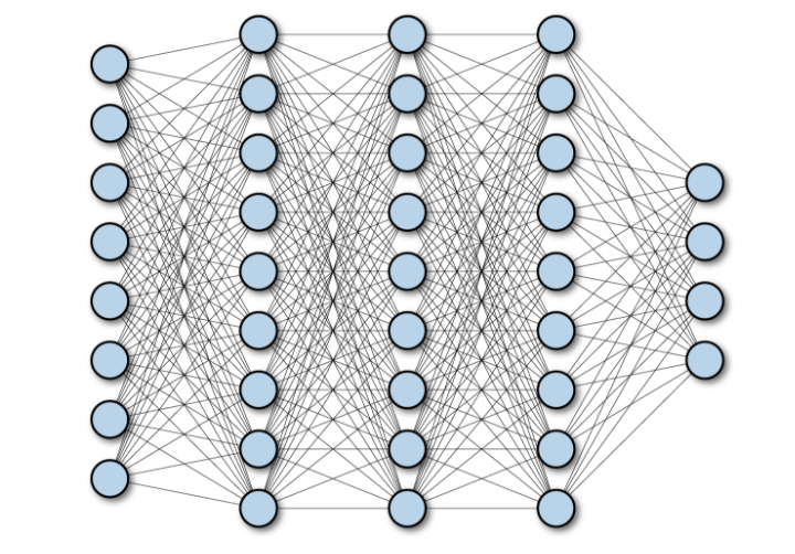
In PyTorch parlance, these are linear layers, and they can be specified via nn.Linear(in_size, out_size). Other frameworks might call them other things (e.g. Flux.jl calls them Dense layers).

Strengths and Weaknesses

FCNs are flexible models that can do well at all sorts of “typical” machine-learning tasks (i.e. classification and regression), and can work with various types of inputs (images, text, etc.). They’re basically the linear regression of the deep learning world (in that they’re foundational models, not in the sense that they’re linear…because they aren’t).

Since FCNs connect all nodes in layer i to all nodes in layer i+1, they can be computationally expensive when used to model large datasets (those with lots of predictors) or when the models themselves have lots of parameters. Another issue is that they don’t have any mechanisms to capture dependencies in the data, so in cases where the inputs have dependencies (image data -> spatial dependenices, time-series data -> temporal dependencies, clustered data -> group dependencies), FCNs may not be the best choice.

Example Model in PyTorch

The code below has a basic implementation of a fully-connected network in PyTorch. I’m using fake data and an arbitrary model architecture, so it’s not supposed to be a great model. It’s more intended to demonstrate a general workflow.

Import Libraries

The main library I need here is torch. Then I’m also loading the nn module to create the FCN as well as some utility functions to work with the data.

#import libraries
import torch
from torch import nn
from torch.utils.data import DataLoader, TensorDataset, random_split

Generate Fake Data

In this step, I’m generating some fake data:

• a design matrix, X,
• a set of ground-truth betas
• the result of \(X * \beta\), y_true
• y_true with some noise added to it, y_noisy

# generate some true data
n = 10000
m = 10

beta = torch.randn(m)
X = torch.randn(n, m)
y_true = torch.matmul(X, beta)
y_noisy = y_true + torch.randn(n)
y_noisy = y_noisy.unsqueeze(1)

In the last step, I have to call unsqueeze() on y_noisy to ensure it’s formatted as a tensor with the correct number of dimensions.

Process Data

Here, I’ll create a Dataset using X and y_noisy, then I’ll do some train/test split stuff and create a Dataloader for the train and test sets.

I should probably create a set of notes on datasets and dataloaders in PyTorch, but for now we’ll just say that dataloaders are utility tools that help feed data into PyTorch models in batches. These are usually useful when we’re working with big data that we can’t (or don’t want to) process all at once.

batch_size = 64

ds = TensorDataset(X, y_noisy)

#splitting into train and test
trn_size = int(.8 * len(X))
tst_size = len(X) - trn_size

trn, tst = random_split(ds, [trn_size, tst_size])

trn_dl = DataLoader(trn, batch_size=batch_size)
tst_dl = DataLoader(tst, batch_size=batch_size)

Defining the Model

Now that the data’s set up, it’s time to define the model. FCN’s are pretty straightforward and are composed of alternating nn.Linear() and activation function (e.g. nn.ReLU()) calls. These can be wrapped in nn.Sequential(), which makes it easier to refer to the whole stack of layers as a single module.

I’m also using CUDA if it’s available.

The model definition has 2 parts:

• defining an __init__() method;
• defining a forward() method.

__init__() defines the model structure/components of the model, and it tells us in the very first line (class FCN(nn.Module)) that our class we’re creating, FCN, is a subclass of (or inherits from) the nn.Module class. We then call the nn.Module init function (super().__init__()) and define what our model looks like. In this case, it’s a fully-connected sequential model. There are 10 inputs into the first layer since there are 10 columns in our X matrix. The choice to have 100 output features is arbitrary here, as is the size of the second linear layer (nn.Linear(100, 100)). The output size of the final layer is 1 since this is a regression problem, and we want our output to be a single number (in a classification problem, this would be size k where k is the number of classes in the y variable).

The forward() method defines the order we should call the model components in. In the current case, this is very straightforward, since we’ve already wrapped all of the individual layers in nn.Sequential() and assigned that sequential model to an object called linear_stack. So in forward(), all we need to do is call the linear_stack().

device = (
    "cuda"
    if torch.cuda.is_available()
    else "cpu"
)

#define a fully connected model
class FCN(nn.Module):
    def __init__(self):
        super().__init__()
        self.linear_stack = nn.Sequential(
            nn.Linear(10, 100),
            nn.ReLU(),
            nn.Linear(100, 100),
            nn.ReLU(),
            nn.Linear(100, 1)
        )

    def forward(self, x):
        ret = self.linear_stack(x)
        return ret
    
model=FCN().to(device)
print(model)

FCN(
  (linear_stack): Sequential(
    (0): Linear(in_features=10, out_features=100, bias=True)
    (1): ReLU()
    (2): Linear(in_features=100, out_features=100, bias=True)
    (3): ReLU()
    (4): Linear(in_features=100, out_features=1, bias=True)
  )
)

We could also define the model like this:

class FCN(nn.Module):
    def __init__(self):
        super().__init__()
        self.l1 = nn.Linear(10, 100)
        self.l2 = nn.Linear(100, 100)
        self.l3 = nn.Linear(100, 1)

    def forward(self, x):
        x = self.l1(x)
        x = F.relu(x)
        x = self.l2(x)
        x = F.relu(x)
        ret = self.l3(x)
        return ret

But that doesn’t feel quite as good to me.

Define a Loss Function and Optimizer

These are fairly straightforward. The loss function is going to be mean squared error (MSE) since it’s a regression problem. There are lots of optimizers we could use, but I don’t think it actually matters all that much here, so I’ll just use stochastic gradient descent (SGD).

loss_fn = nn.MSELoss()
opt = torch.optim.SGD(model.parameters(), lr=1e-3)

Define a Train Method

Now we have a model architecture specified, we have a dataloader, we have a loss function, and we have an optimizer. These are the pieces we need to train a model. So we can write a train() function that takes these components as arguments. Here’s what this function could look like:

def train(dataloader, model, loss_fn, optimizer):
    #just getting the size for printing stuff
    size = len(dataloader.dataset)
    #note that model.train() puts the model in 'training mode', which allows for gradient calculation
    #model.eval() is its contrasting mode
    model.train()
    for batch, (X, y) in enumerate(dataloader):
        X, y = X.to(device), y.to(device)

        #compute error
        pred = model(X)
        loss = loss_fn(pred, y)

        #backprop
        loss.backward()
        optimizer.step()
        optimizer.zero_grad()

        if batch % 10 == 0:
            loss, current = loss.item(), (batch + 1) * len(X)
            print(f"loss: {loss:>5f} [{current:>5d}/{size:>5d}]")

Let’s walk through this:

• We get size just to help with printing progress
• model.train() puts the model in “train” mode, which lets us calculate the gradient
• We then iterate over all of the batches in our dataloader…
• We move X and y to the GPU (if it’s available)
• Make predictions from the model
• Calculate the loss (using the specified loss function)
• Calculate the gradient of the loss function for all model parameters (via loss.backward())
• Update the model parameters by applying the optimizer’s rules (optimizer.step())
• Zero out the gradients so they can be calculated again (optimizer.zero_grad())
• Then we do some printing at the end of the loop to show our progress.

Define the Test Method

Unlike the train() function we just defined, test() doesn’t do parameter optimization – it simply shows how well the model performs on a holdout (test) set of data. This is why we don’t need to include the optimizer as a function argument – we aren’t doing any optimizing.

Here’s the code for our test() function:

def test(dataloader, model, loss_fn):
    size = len(dataloader.dataset)
    #set model into eval mode
    model.eval()
    test_loss = 0

    #set up so we're not calculating gradients
    with torch.no_grad():
        for X, y in dataloader:
            X, y = X.to(device), y.to(device)
            pred = model(X)
            test_loss += loss_fn(pred, y).item() * X.size(0)
    avg_loss = test_loss / size
    print(f"Avg Loss: {avg_loss:>7f}\n")

And we can walk through it:

• In this function, size is actually useful in calculating our loss. We have to do some kinda wonky slight-of-hand when estimating the model loss here. We are using mean-squared error (MSE) as our loss function, and for each batch in the dataloader, it will give us the mean-squared error (a single number per batch). We then multiply this average loss by the size of the batch to get the “total” loss per batch, and we sum up all of the total batch losses to get the total overall loss (test_loss in the function). Since this is the total loss, we then have to divide by the number of observations to get us back to the mean squared error.
• model.eval() puts the model into evaluation mode, signaling that we’re not going to be calculating gradients or anything like that.
• We initialize test_loss to 0
• Then for the remainder, we make predictions (just like we did in the train() function) and calculate loss as described in the first bullet point above.

Train the Model

Now we can finally train the model. We’ll train over 5 “epochs”, i.e. 5 passes through the full dataset. This is arbitrary here – in real-world contexts this is a number we probably want to tune for or at least choose carefully.

We do the traning with a simple for loop, and during each iteration through the loop we:

1. train the model;
2. show the performance on the test set

Since we included some print statements in our train() and test() functions, we can monitor the progress of our model’s training.

epochs = 5
for i in range(epochs):
    print(f"Epoch {i+1}\n------------------")
    train(trn_dl, model, loss_fn, opt)
    test(tst_dl, model, loss_fn)
print("Done!")

Epoch 1
------------------
loss: 11.559361 [   64/ 8000]
loss: 10.150082 [  704/ 8000]
loss: 12.431366 [ 1344/ 8000]
loss: 8.781148 [ 1984/ 8000]
loss: 11.217168 [ 2624/ 8000]
loss: 8.060587 [ 3264/ 8000]
loss: 9.669640 [ 3904/ 8000]
loss: 9.624810 [ 4544/ 8000]
loss: 9.808482 [ 5184/ 8000]
loss: 10.177684 [ 5824/ 8000]
loss: 8.251064 [ 6464/ 8000]
loss: 7.369075 [ 7104/ 8000]
loss: 8.711451 [ 7744/ 8000]
Avg Loss: 9.769837

Epoch 2
------------------
loss: 10.468843 [   64/ 8000]
loss: 9.218903 [  704/ 8000]
loss: 11.100779 [ 1344/ 8000]
loss: 7.746999 [ 1984/ 8000]
loss: 9.873242 [ 2624/ 8000]
loss: 7.149283 [ 3264/ 8000]
loss: 8.435396 [ 3904/ 8000]
loss: 8.367870 [ 4544/ 8000]
loss: 8.155600 [ 5184/ 8000]
loss: 8.412899 [ 5824/ 8000]
loss: 6.608739 [ 6464/ 8000]
loss: 5.931441 [ 7104/ 8000]
loss: 6.928466 [ 7744/ 8000]
Avg Loss: 7.608491

Epoch 3
------------------
loss: 7.947855 [   64/ 8000]
loss: 7.037781 [  704/ 8000]
loss: 8.046132 [ 1344/ 8000]
loss: 5.375796 [ 1984/ 8000]
loss: 6.869387 [ 2624/ 8000]
loss: 4.945308 [ 3264/ 8000]
loss: 5.555494 [ 3904/ 8000]
loss: 5.423590 [ 4544/ 8000]
loss: 4.637858 [ 5184/ 8000]
loss: 4.751605 [ 5824/ 8000]
loss: 3.392872 [ 6464/ 8000]
loss: 2.943655 [ 7104/ 8000]
loss: 3.505284 [ 7744/ 8000]
Avg Loss: 3.615225

Epoch 4
------------------
loss: 3.360711 [   64/ 8000]
loss: 3.129750 [  704/ 8000]
loss: 3.220852 [ 1344/ 8000]
loss: 2.028703 [ 1984/ 8000]
loss: 2.811476 [ 2624/ 8000]
loss: 2.152989 [ 3264/ 8000]
loss: 2.169516 [ 3904/ 8000]
loss: 2.104460 [ 4544/ 8000]
loss: 1.674014 [ 5184/ 8000]
loss: 1.971039 [ 5824/ 8000]
loss: 1.329351 [ 6464/ 8000]
loss: 1.101499 [ 7104/ 8000]
loss: 1.521148 [ 7744/ 8000]
Avg Loss: 1.489543

Epoch 5
------------------
loss: 1.216901 [   64/ 8000]
loss: 1.191105 [  704/ 8000]
loss: 1.300725 [ 1344/ 8000]
loss: 0.935616 [ 1984/ 8000]
loss: 1.545732 [ 2624/ 8000]
loss: 1.388198 [ 3264/ 8000]
loss: 1.273956 [ 3904/ 8000]
loss: 1.170510 [ 4544/ 8000]
loss: 1.217884 [ 5184/ 8000]
loss: 1.544257 [ 5824/ 8000]
loss: 1.180285 [ 6464/ 8000]
loss: 0.944844 [ 7104/ 8000]
loss: 1.244212 [ 7744/ 8000]
Avg Loss: 1.219065

Done!

And that’s a complete step-by-step for a fully-connected neural net!